- 1 Theoretical Background
- 2 The Fundamental Design Challenge: Comparing Apples and Oranges
- 3 The Origin Story of the Experimental Design
- 4 Revisiting Reasons for Data Exclusion
- 5 Counterbalance Fail
- 6 Back to Apples and Oranges: How to Compare Learning Curves Between Tasks
- 7 Statistical Analyses
- 8 Summary
This R Markdown documents the key analyses reported in the article “Acetaminophen Enhances the Reflective Learning Process” by Rahel Pearson, Seth Koslov, Bethany Hamilton, Jason Shumake, Charles S. Carver, and Christopher G. Beevers.1 It is written from my perspective as a co-author who was not involved in designing or conducting the study but was consulted after it was finished to help with the data analysis. As Fisher famously said, “To consult the statistician after an experiment is finished is often merely to ask him to conduct a post mortem.”
While these data were not dead on arrival, the experimental design presented several challenges. Some were readily apparent at the time, and some have only recently come to light during an extensive data audit I performed in response to a scathing critique of the study’s analysis procedures. I found that nearly all of the points raised in this critique are without merit, but I am grateful to it in one sense: it prompted me to take a much closer look at this project than I otherwise would have because, to be honest, I had always regarded it as a low-priority consulting job of not much consequence. But because I took a closer look, I discovered a problem (unrelated to any points in that critique) that definitely requires redressing.
This post will be a complete and transparent account of how this study was planned and conducted, every problem encountered, and every solution implemented. I will show the R code that reproduces the analyses reported in the published article, as well as new supplemental analyses. I encourage you to download the data files from our repository. If you set data_path (first line in the following code chunk) to your local path containing the downloaded files, you can reproduce all of the following output for yourself in R.
data_path <- "~/Box/apap_verse"
library(tidyverse); library(DT)
reflective_data <- read_csv(
  paste(data_path, "datasetRB.csv", sep = "/"),
  col_types = cols_only(
    sub = col_factor(levels = 101:200), # participant ID
    trial = col_integer(), # trial number, 1-150
    acc = col_integer(), # accuracy: 1 if `resp` matches `corr.resp`, else 0
    count.n = col_integer(), # running count of consecutive correct responses
    rule.n = col_integer(), # cumulative sum of rule switches
    bottle = col_character(), # treatment: "active" = acetaminophen
    order = col_integer(), # task order: did this task come first or second?
    feature = col_character(), # stimulus set used for task: houses or vehicles
    Condition = col_integer() # one of four task-admin conditions that is the
                              # cross-product of task order and stimulus set
  )
  # `rule.n` as it appears in the data set increments on the same trial that
  # `count.n` reaches 10, but it should actually increment on the next trial;
  # e.g., the 10th consecutive correct response for Rule 1 is currently marked
  # as the first trial of Rule 2, but it is really the last trial of Rule 1.
  # The following line of code corrects this.
) %>% mutate(rule.n = factor(ifelse(count.n == 10, rule.n - 1, rule.n)),
             condition = factor(Condition, levels = 1:4, labels = c(
               "reflective first with vehicles",
               "reflexive first with vehicles",
               "reflective first with houses",
               "reflexive first with houses")))
reflexive_data <- read_csv(
  paste(data_path, "datasetII.csv", sep = "/"),
  col_types = cols_only(
    sub = col_factor(level = 101:200), # participant ID
    trial = col_integer(), # trial number, 1-150
    acc = col_integer(), # accuracy: 1 if `resp` matches `corr.resp`, else 0
    count.n = col_integer(), # running count of consecutive correct responses
    bottle = col_character(), # treatment: "active" = acetaminophen
    order = col_integer(), # task order: did this task come first or second?
    feature = col_character(), # stimulus set used for task: houses or vehicles
    Condition = col_integer() # one of four task-admin conditions that is the
                              # cross-product of task order and stimulus set
  )
) %>% mutate(condition = factor(Condition, levels = 1:4, labels = c(
               "reflective first with vehicles",
               "reflexive first with vehicles",
               "reflective first with houses",
               "reflexive first with houses")))
# reduce to relevant variables and dummy code tx and task
reflexive_task <- reflexive_data %>%
  mutate(tx = as.integer(bottle == "active"), task = 0) %>%
  select(sub, tx, task, trial, acc, order, feature, condition)
reflective_task <- reflective_data %>%
  mutate(tx = as.integer(bottle == "active"), task = 1) %>%
  select(sub, tx, task, rule.n, trial, acc, order, feature, condition)
1 Theoretical Background
This is explained in much greater detail in our article, but the basic idea behind this study stems from theoretical work emphasizing the contribution of serotonin to the balance between two modes of self-regulation, namely the Competition between Verbal and Implicit Systems (COVIS) model of learning and decision making. My co-authors’ hypothesis is that serotonin biases neural systems toward reflective learning at the expense of reflexive learning. This passage from the paper explains the difference between reflective and reflexive learning:
Categorization on reflective-optimal tasks depends on logical reasoning processes (e.g. hypothesis testing). Rules on these tasks are easily verbalized and individuals maximize accuracy by using an explicit hypothesis and iterative hypothesis updating to guide categorization. For example, rule-based categorization tasks like the oft-used Wisconsin Card Sorting Task (WCST) are thought to rely on reflective learning processes (Hélie et al., 2012). In contrast, categorization learning on reflexive-optimal tasks depends on intuitive processing and cumulative, incremental reinforcement learning. Rules on these tasks are not easily verbalized. Accuracy on reflexive-optimal tasks is maximized by integrating high-level perceptual details (e.g. height and color) at a pre-decisional stage and associating those percepts with rewarding motor actions.
So if the objective was to enhance serotonin transmission, why give participants acetaminophen? Why not give them an SSRI like Celexa?
The answer is, in a word, convenience.
Investigational use of a prescription drug poses several logistical hurdles: needing a special license and a supervising physician, heightened IRB scrutiny, and probably greater difficulty recruiting volunteers. There is evidence, reviewed in the article, that acetaminophen transiently enhances serotonin function. Of course, acetaminophen has a lot of other effects, too, so the downside is that its actions are not specific to the serotonin system. But the upside is that it avoids the various logistical hurdles of administering a prescription SSRI.
2 The Fundamental Design Challenge: Comparing Apples and Oranges
My co-authors hypothesized that, if acetaminophen increases serotonin signaling, then this should produce a greater within-person difference between performance on a reflexive learning task vs. a reflective learning task, in the direction of enhancing reflective processing and impairing reflexive processing. So the basic plan was to give each person a reflexive task and a reflective task, and then test for a treatment \(\times\) task interaction.
Sounds easy enough, but here’s the problem. Reflexive learning is slow and characterized by incremental progress, whereas reflective learning is fast and characterized by sudden insights. As we will see, half of this sample was able to master the first reflective rule in 10-14 trials, the other half in 15-45 trials. In contrast, less than half of the sample was able to master the reflexive task even after 150 trials.
In designing their experiment, my co-authors focused on matching the time that the participants spent on each task, so whenever the participants mastered a reflective rule (defined in advance as getting 10 correct responses in a row), they were given a new rule to learn, and this process was repeated until 150 trials (same as the reflexive task) had been completed. That certainly succeeds in matching the two tasks in terms of number of total trials, but this doesn’t come for free.
Namely, whereas the reflexive task contains a single learning curve, the reflective task now contains a variable number of multiple learning curves. If one were to aggregate data across all trials, participants who are especially good at the reflective task will be made to look artificially worse because they keep having to start over: effectively, every time a person achieves 100% performance, this triggers the introduction of a bunch of 50% performance trials into their overall time series. (See section Overall Accuracy for some concrete examples of this.) Moreover, the nature of the learning process itself undergoes a significant shift after the first rule is acquired because the participant is no longer just learning a new rule but also having to “unlearn” an old rule.
To make these points more concrete, here are three examples of individuals’ learning curves for the two different tasks. I generated these curves by fitting a loess smooth to the time series of Boolean values that indicate whether the participant was correct or not on each individual trial. The first plot shows that learning on the reflexive task is very gradual over the course of the 150 trials. The first person stays at chance performance for the first 100 trials, at which point linear improvement starts to occur. The other examples start improving gradually right away and reach asymptotic performance by trial 100.
reflexive_examples <- reflexive_task %>% filter(sub %in% c(101, 105, 110))
ggplot(reflexive_examples, aes(x = trial, y = acc)) +
  ylab("accuracy") +
  facet_grid(sub~.) + ggtitle("Reflexive Task") +
geom_smooth(method = "loess", se = FALSE, span = .5) + theme_classic() 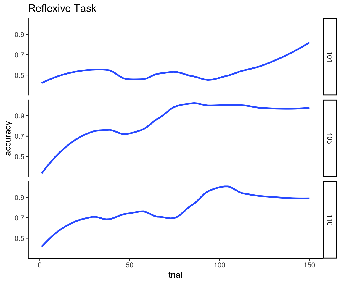
The next plot for the reflective task shows why we can’t just directly compare the performance curves across all 150 trials because, quite simply, the time series for the reflective task is not a single acquisition curve. You can see clearly here the point made earlier about the variable number of acquisition curves in which each person improves to perfect performance, falls off to chance performance, improves again, falls off again, and so on. You can further see that acquiring the second and subsequent rules is categorically harder than acquiring the first rule because the memory of the old rule interferes with acquiring the new one. And there are a lot of individual differences in the ability to keep adapting to these rule switches.
reflective_examples <- reflective_task %>% filter(sub %in% c(101, 105, 110))
ggplot(reflective_examples, aes(x = trial, y = acc, color = rule.n)) +
  facet_grid(sub~.) + ggtitle("Reflective Task") + ylab("accuracy") +
  geom_smooth(method = "loess", se = FALSE, span = .5) + theme_classic() +
  coord_cartesian(ylim = c(0,1))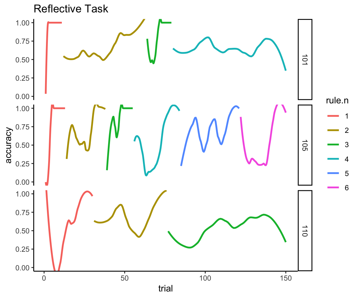
I think we also see (in the examples of participants 101 and 110) that participants can start to get tired or bored the longer this task drags on, as evidenced by spending the last half of the session hovering around chance (50%) performance. Given that task difficulty has not changed, I assume that fatigue/boredom is a more likely explanation than that the participants have lost their ability to learn. Thus, during the latter half of this task, sustained attention and motivation are probably much bigger determinants of performance than they are at the beginning of the task. If you think this might be a problem for interpreting the results, this is why the authors planned to exclude participants who were predominantly random responders.
3 The Origin Story of the Experimental Design
So at this point you might be wondering, if the authors were interested in analyzing differences in acquisition between the two tasks, why didn’t they just collect data for one reflective rule and then simply normalize the learning curves for the different number of trials when comparing them?
First of all, it is important to understand that this design was not their first choice but rather something of a last resort. Their initial plan was to assess a single acquisition curve for a reflective task, but, because they were planning a within-person comparison to the reflexive task, they needed both tasks to be equally challenging. This is important because the two tasks are supposed to be counterbalanced: half of the participants get the reflexive task before the reflective, and half get reflective before reflexive. They needed the tasks to be of equal length and difficulty to insure that participants who got the reflexive task last started it with the same amount of mental fatigue and acetaminophen levels as those who started the reflective task last. That’s why they couldn’t just use the same reflective task as in prior work—it’s too easy. So why not just come up with a more challenging reflective task that would still result in a single learning curve?
Well, that’s exactly what they tried to do at first. Co-author SK spent a laudable amount of time and effort developing and testing new reflective tasks, and he had some success in obtaining learning curves that were more comparable to those of the reflexive task. But what he came to realize was that the reflective task had become so complex that he could no longer be certain that participants were still using a reflective strategy to solve it; they might have switched over to a reflexive strategy, in which case we would have just ended up comparing two reflexive tasks.
And so my co-authors arrived at their final experimental design. So that there would be no ambiguity about the reflective vs. reflexive nature of the tasks, they decided to use the original (easy) reflective task. But then, to match the overall difficulty and length of the experimental sessions, they introduced the rule switches. As they have explained their thinking to me, they were fully aware that set-shifting is not equivalent to category learning, but they also didn’t think it was that far of a step to go from using one rule to multiple rules to assess reflective learning. Besides, they reasoned, they could still look at just the first rule to derive a “pure” measure of reflective learning.
And their analysis plan was just that: use trials-to-criterion and learning-curve analyses for just the first reflective rule, thus replicating the approach used in their previous study. In addition, they introduced the new approach of measuring accuracy across multiple rule switches.
Had I been involved in the design of this study, there are a few things I would have pointed out. First, I can see why going from a single rule to multiple rules might seem like a small step, but, from my vantage point (having done research on extinction and reversal learning), it’s a bigger neurocognitive leap than one might imagine to learn one thing and then learn another thing that reverses the first thing.
Nonetheless, I’m on board with the need to match the tasks for aggregate time and effort, and I agree the rule switches seem like the best option for accomplishing that (given that the effort to develop a different task didn’t work out). But there is one thing I would have changed: I wish my co-authors had used a fixed number of trials for a fixed number of rules (e.g., 15 trials for the first rule and 45 trials each for 3 subsequent rules) instead of having the number of rules and trials per rule vary depending on individual learning rates. It’s not the end of the world that they didn’t, but it would have made the analysis easier. I will explain why in the sections that follow. But first, I need to relay some important additional information, some of which I have only recently uncovered.
4 Revisiting Reasons for Data Exclusion
Our published methods state the following regarding data exclusions: “Six participants (four active and two placebo) were excluded from analyses because they lacked complete task data, and seven participants (five active and two placebo) were excluded from analyses because their category-task performance was at or below chance (≤50%).” Before we proceed, I want to provide more details about these exclusions and critically evaluate their necessity.
4.1 Problems with task administration
When I was first provided the data to conduct my own analysis, I was given the following line of code by co-author BH identifying participant IDs that should be dropped because of “issues in task”:
#bad IDS due to issues in task. There are 5 IDS
badIDs <- c(114,151,171,190,200)
There is additionally one participant, ID = 103, who is missing altogether from the data set because this individual fell asleep during the first task and then dropped out of the study. The 5 participants with task issues plus the 1 participant who withdrew from the study correspond to what our publication reports as 6 participants who were “excluded from analyses because they lacked complete task data”.
While 6 individuals were indeed excluded because of issues related to task completion, this statement was, regrettably, uninformative as to what those issues were. As mentioned, one of these participants does not just lack complete task data—they lack data altogether because they went to sleep. As for the other 5 people, I discovered during my audit that they do have complete data for the reflective and reflexive learning tasks; apparently the “issues in task” occurred during tasks that were administered before the learning tasks, during the ~60-minute window after acetaminophen/placebo was administered while waiting for the drug to take effect.
This was news to me that additional data (other than the demographic info reported in our publication) had been collected. It appears that the purpose of these other tasks was to make the most of the participants’ time—instead of just having them wait around doing nothing for an hour, why not take advantage of that time to pilot some other tasks?
On the one hand, I can see why my co-authors didn’t think this worth mentioning—none of these data influenced the analysis of the subsequent learning tasks,2 nor could the data be used to look for other acetaminophen effects (at least not without controversy) because of, you know, pharmacokinetics.
On the other hand, these details might be important for understanding and replicating the results. (Might fatigue from the preceding tasks be an important moderating factor?) What’s more, they are important for understanding the notes memorializing why certain participants were excluded. So here is the timeline of the full experimental protocol, which I pulled from the authors’ IRB protocol:
| Start (minutes) | Finish (minutes) | Element |
|---|---|---|
| 0 | 5 | Admin drug/placebo |
| 5 | 20 | Affective flanker |
| 20 | 30 | Stroop |
| 30 | 40 | Questionnaires |
| 40 | 55 | Affective flanker |
| 55 | 65 | Stroop |
| 65 | 75 | Reflective or reflexive task |
| 75 | 85 | Reflective or reflexive task |
| 85 | 90 | Pay and debrief |
And now here are summaries of the experimenters’ notes on each of the excluded participants. All of these refer to issues that occurred with the affective flanker or Stroop tasks mentioned in the above table.
- 114: IT network server maintenance caused tasks to lag and take twice as long.
- 151: Participant restarted after 10 min because numlock was on, resulting in erroneous feedback.
- 171: Computer crashed 30 min into experiment; experiment was restarted.
- 190: Computer crashed 40 min into experiment; experiment was restarted.
- 200: Task interrupted by fire drill.
These events delayed the start of the learning tasks by anywhere from 15 minutes to 1 hour. Co-authors BH and SK who made the call to exclude these participants don’t recall their exact reasoning (this happened over 2 years ago), but it seems there was concern that blood levels of acetaminophen would be different from the other participants because of the delays. Moreover, these participants had unusual, frustrating experiences in the hour leading up to the key experiment, which could have an unknown impact on their subsequent performance on the learning tasks.
However, peak plasma levels of acetaminophen actually occur 90 minutes after ingestion, and its half-life is 1.5-2.5 hours. So while blood levels might be somewhat different for these participants, the delays were not long enough to lead to substantial washout; on the contrary, blood levels could have been somewhat higher (and of course this isn’t an issue for the placebo recipients). And, while the participants did have unusual and likely frustrating experiences during their waiting period, the learning tasks themselves appear to have been administered without incident. Therefore, I think it is appropriate to reanalyze the data without excluding these participants to evaluate whether or not this makes a substantive difference in the results.
4.2 Random responding
It is customary practice in behavioral/social sciences research to have some criterion for identifying and excluding random responders. (See for example Random Responding from Participants is a Threat to the Validity of Social Science Research Results.)
The criterion used by my colleagues was to exclude anyone who failed to show above-chance accuracy after averaging across all 150 trials on either learning task:
reflex_exclude <- (reflexive_task %>% group_by(sub) %>%
  summarize(meanAcc= mean(acc)) %>%
  filter(meanAcc <= .50))$sub
reflect_exclude <- (reflective_task %>% group_by(sub) %>%
  summarize(meanAcc= mean(acc)) %>%
  filter(meanAcc <= .50))$sub
to_exclude <- list(
  reflexive = as.character(reflex_exclude),
  reflective = as.character(reflect_exclude)
)
to_exclude
## $reflexive
## [1] "107" "147" "157" "159" "168" "179"
##
## $reflective
## [1] "156"This leads to 6 individuals being excluded because of chance-level performance on the reflexive task and 1 individual being excluded because of chance-level performance on the reflective task, for a total of 7 participants who were excluded for presumed lack of task engagement/motivation. This was the a priori exclusion criterion set by my co-authors who planned and ran this experiment, so I followed it for my analyses as well. But I do want to acknowledge that other choices could have been made.
On the one hand, I could make the argument that if our goal is to eliminate random responding, then this criterion doesn’t go nearly far enough. Random responders should be near 50% accuracy, but not necessarily at or below it; requiring at least 55% accuracy might make more sense. Also, this criterion does nothing to address the problem we saw above where participants may start out engaged and providing good data but eventually get tired or bored and start providing bad data.
On the other hand, notice how all but one of the excluded participants was excluded based on their poor performance on the reflexive task. Unlike the reflective task, the reflexive task is legitimately difficult, and it is plausible to me that some individuals might remain at chance performance despite adequate task engagement. This is especially true if acetaminophen impaired performance on this task as hypothesized.
4.3 Parallel reanalysis
Given that there is a reasonable case to be made for including all participants, I will create two data sets: one that excludes the 12 participants identified above (and reproduces the key analyses reported in our article) and one that includes all participants with data. (There is nothing I can do about the one participant who has no data.) In the analyses that follow, I will evaluate how much the results change when we do not exclude any participants.
to_exclude <- unlist(c(to_exclude, task_prob = badIDs))
reflect_no_exclude <- reflective_task %>% filter(rule.n == 1) %>%
  select(-rule.n)
reflect_with_exclude <- reflective_task %>%
  filter(rule.n == 1, !sub %in% to_exclude) %>% select(-rule.n)
reflex_no_exclude <- reflexive_task
reflex_with_exclude <- reflexive_task %>% filter(!sub %in% to_exclude)
n_orig = n_distinct(reflect_no_exclude$sub)
n_after_exclude <- n_distinct(reflect_with_exclude$sub)
5 Counterbalance Fail
Now we arrive at the newly discovered problem that I mentioned in the introduction. So recall from the discussion of the experimental design that task order was supposed to be counterbalanced, meaning that, within each treatment group, the number of participants who get the reflective task before the reflexive task should be equal to the number who get the reflexive task before the reflective task. In addition, my co-authors also tried to balance the stimuli sets (pictures of either houses or vehicles) used for each task, so there was a product of 4 conditions that needed balancing:3
levels(reflexive_task$condition)## [1] "reflective first with vehicles" "reflexive first with vehicles"
## [3] "reflective first with houses" "reflexive first with houses"So I was certainly aware of this aspect of the design, and “order” and “feature” variables were in the data set I was provided (which was exactly the same as what you are seeing here). I seem to remember someone asking me if condition should be included in our models as a potential moderator of treatment effect; I definitely remember rejecting that idea because the sample size struck me as inadequate. Modeling a 2 \(\times\) 4 (treatment \(\times\) task condition) interaction with a sample size of 100 would result in an N of only 12-13 per cell, and that seems like a recipe for overfitting the data. For this reason, I thought it best to leave potential effects of condition as part of the overall error term rather than attempt to model them. However, this was couched on the assumption that the conditions actually were counterbalanced, such that any measurement variance due to condition would be independent of treatment. The thought never crossed my mind that the conditions might not actually be counterbalanced.
Then, while constructing this document to accompany the public release of these data, I wanted to list the \(N\) per condition when describing the dummy coding for the Condition variable. I still had not fathomed that the conditions might be unbalanced; I was just trying to be thorough in documenting the data set for our public repository. But then I found this:
design <- reflect_no_exclude %>%
  select(sub, tx, order, feature, condition) %>% distinct %>%
  mutate(task_order = factor(
    order, labels = c("reflective first", "reflexive first"))) %>%
  select(-order)
condition_table <- with(design, table(condition, tx))
condition_table
## tx
## condition 0 1
## reflective first with vehicles 10 15
## reflexive first with vehicles 15 10
## reflective first with houses 10 14
## reflexive first with houses 15 10Now that doesn’t look too bad on the surface; a perfect counterbalance would be 12.5 per cell (100 does not divide evenly by 8), so we should expect 12s and 13s and perhaps one 11 (given that we’re missing one participant who fell asleep). This doesn’t seem that far off from that expectation. Indeed, if assignment to condition is perfectly random we should expect to see a configuration as extreme as this about 31% of the time:
fisher.test(condition_table)##
## Fisher's Exact Test for Count Data
##
## data: condition_table
## p-value = 0.3128
## alternative hypothesis: two.sidedBut if you look more closely, the imbalance in condition assignment is not being distributed equally across task order and stimulus feature. In fact, stimulus feature is perfectly balanced within each treatment group:
feature_table <- with(design, table(feature, tx))
feature_table
## tx
## feature 0 1
## houses 25 24
## vehicle 25 25fisher.test(feature_table)##
## Fisher's Exact Test for Count Data
##
## data: feature_table
## p-value = 1
## alternative hypothesis: true odds ratio is not equal to 1
## 95 percent confidence interval:
## 0.4401812 2.4656794
## sample estimates:
## odds ratio
## 1.041262All of the imbalance is borne by task order:
order_table <- with(design, table(task_order, tx))
order_table
## tx
## task_order 0 1
## reflective first 20 29
## reflexive first 30 20fisher.test(order_table)##
## Fisher's Exact Test for Count Data
##
## data: order_table
## p-value = 0.07134
## alternative hypothesis: true odds ratio is not equal to 1
## 95 percent confidence interval:
## 0.190428 1.104389
## sample estimates:
## odds ratio
## 0.46348445.1 Why is this a problem (potentially)?
This failure to fully counterbalance task order within treatment condition introduces an unintended partial confound between order effects (such as they exist) and treatment effects. It is a plausible hypothesis that participants will do somewhat worse on the second task because they have to shift away from the strategy that they got accustomed to on the first task, and this raises the possibility that the treatment effects reported in our manuscript might be, in whole or in part, driven by order effects. This is a possibility that we cannot ignore, but nor should we jump to the conclusion that there is no treatment effect based on the mere existence of this confound. It all depends on whether or not there is an order effect and how strong it is, and whether or not the results substantively change when we statistically correct for the counter-imbalance. Before I talk about my strategy for doing just that, I want us to understand what went wrong so that we and anyone else reading this can prevent this sort of thing from happening in the future.
5.2 What went wrong?
According to Fisher’s exact test, there is only a 7% chance of this degree of imbalance occurring under a completely randomized assignment, but, importantly, this is not something that should be left completely to chance in the first place. Before I perform the “autopsy” to figure out what went wrong, it is important to understand what should have gone right. In a situation like this, when it is important to achieve an equal N per cell, it is preferable to use pseudorandom assignment. Here’s an easy way to do this in R.
First off, recognize that there are 4 task conditions that need balancing across 2 treatment groups, so the lowest common denominator in the sequence of treatment assignment is 4 \(\times\) 2 = 8. So we can only achieve complete balance over a block of 8 participants or 16 participants or 24 participants and so on, and we should likewise plan for a sample size that is a multiple of whatever block size we decide. Let’s say we want to keep every 8 participants balanced across a planned sample of 104 participants. Then we write a function to return a balanced sequence of treatment assignments across the conditions:
get_balanced_block <- function(tx, cond, blocksize){
# throw an error if someone tries to randomize a block size that cannot
# be balanced
if(blocksize %% (length(cond) * length(tx)) != 0){
stop("Size must be a multiple of the number of conditions and treatments")
}
block <- expand.grid(cond = cond, tx = tx)
if(nrow(block) < blocksize){
times <- blocksize / nrow(block)
block <- map(1:times, ~ block) %>% reduce(bind_rows)
}
sample_frac(block)
}
set.seed(42)
block_size <- 8
sample_size <- 104
tx_assignments <- bind_cols(
sub = 1:sample_size,
replicate(sample_size/block_size,
get_balanced_block(tx = 0:1, cond = 1:4, blocksize = block_size),
simplify = FALSE) %>%
reduce(bind_rows)
)
datatable(tx_assignments, rownames = FALSE)The basic algorithm is simple: 1) construct a completely balanced condition \(\times\) treatment assignment table for a block of 8; 2) randomly shuffle the rows of the table; 3) repeat until an assignment is obtained for every person. In this way you get an overall random(ish) assignment sequence while also guaranteeing this:
with(tx_assignments, table(cond, tx))## tx
## cond 0 1
## 1 13 13
## 2 13 13
## 3 13 13
## 4 13 13Even under the scenario where one person falls asleep and drops out and we only go up to 100 participants (and not the more ideal multiple of 8 that is 104), this is what we should have seen under a more optimal treatment randomization algorithm:
with(tx_assignments[c(1:2, 4:100),], table(cond, tx))## tx
## cond 0 1
## 1 13 12
## 2 13 12
## 3 12 12
## 4 13 12Whoever came up with the treatment assignment sequence for this study appears to have implemented a different approach that almost works—but unfortunately only up to a point:
display_design <- tibble(
sub = 101:200,
cond = rep(1:4, times = 25),
# inserting the treatment assignment for the participant who dropped out
# so that you can better see the pattern of the intended sequence
tx = c(design$tx[1:2], 1, design$tx[3:99])
)
datatable(display_design, rownames = FALSE)First, note that condition assignment is a fixed repeating sequence of {1,2,3,4}, and treatment assignment starts off as a pair of alternating sequences of length 4: {1,0,1,0} followed by {0,1,0,1}. While this is not random, it does succeed in balancing treatment and condition assignments for a block of 8, in the same way that the assignments I created above are balanced. So at a cursory glance everything looks fine, and indeed it is fine for the first 16 participants:
with(display_design[1:16,], table(cond, tx))## tx
## cond 0 1
## 1 2 2
## 2 2 2
## 3 2 2
## 4 2 2It’s right after this that the counterbalancing starts to go off the rails. Note the next block of 8 participants is not balanced:
display_design[17:24,]## # A tibble: 8 x 3
## sub cond tx
## <int> <int> <dbl>
## 1 117 1 1
## 2 118 2 0
## 3 119 3 1
## 4 120 4 0
## 5 121 1 1
## 6 122 2 0
## 7 123 3 1
## 8 124 4 0Instead of continuing to repeat the randomization in blocks of 8, it appears to have been stopped at 20, leaving 4 participants unmatched. Then the same imbalanced sequence of 20 was repeated 5 more times, so the imbalance in task order grew wider with each block of 20 participants, eventually becoming 5 times as large:
x <- list(`After 20 participants` = 19,
`After 40 participants` = 39,
`After 60 participants` = 59,
`After 80 participants` = 79,
`After 100 participants` = 99)
map(x, ~ with(design[1:.x,], table(task_order, tx)))## $`After 20 participants`
## tx
## task_order 0 1
## reflective first 4 5
## reflexive first 6 4
##
## $`After 40 participants`
## tx
## task_order 0 1
## reflective first 8 11
## reflexive first 12 8
##
## $`After 60 participants`
## tx
## task_order 0 1
## reflective first 12 17
## reflexive first 18 12
##
## $`After 80 participants`
## tx
## task_order 0 1
## reflective first 16 23
## reflexive first 24 16
##
## $`After 100 participants`
##                   tx
## task_order          0  1
##   reflective first 20 29
## reflexive first 30 20So there were two causes of the imbalance: 1) not continuing the randomization throughout the entire sequence of participants but rather repeating a sequence multiple times and, more problematic, 2) repeating a sequence that was not balanced and could not be balanced because the length of the sequence (20) is not a multiple of 8.
5.3 How do we fix it?
In addition to the parallel reanalysis of the full and reduced samples, I will further reanalyze the data to adjust for the unequal treatment \(N\) between task orderings. For R functions that support it (e.g., methods that inherit class “lm” or “glm”), my preferred correction technique is to use a weighting adjustment. This is far more common in survey research than in experimental research, but the principle is exactly the same: persons in an underrepresented category get a weight larger than 1 and persons in an over-represented category get a weight smaller than 1. Here, we choose observation weights that will equalize the influence of the two different task orders when a model of treatment effect is being fit. We need to do this separately for the complete data set and the data set with participant exclusions because the degree of imbalance is different.
5.3.1 Correction weights for data with participant exclusions
design_with_exclude <- design %>%
  filter(!sub %in% to_exclude) %>%
  group_by(tx, task_order) %>%
  mutate(wt = n_after_exclude/4/n())
design_with_exclude %>% summarize(N = n(), weight = wt[1]) %>%
  mutate(`Effective N` = N * weight)
## # A tibble: 4 x 5
## # Groups: tx [2]
## tx task_order N weight `Effective N`
## <int> <fct> <int> <dbl> <dbl>
## 1 0 reflective first 18 1.21 21.8
## 2 0 reflexive first 28 0.777 21.8
## 3 1 reflective first 24 0.906 21.8
## 4 1 reflexive first 17 1.28 21.8design_with_exclude <- ungroup(design_with_exclude)5.3.2 Correction weights for data without participant exclusions
design_no_exclude <- design %>%
  group_by(tx, task_order) %>%
  mutate(wt = n_orig/4/n())
design_no_exclude %>% summarize(N = n(), weight = wt[1]) %>%
  mutate(`Effective N` = N * weight)
## # A tibble: 4 x 5
## # Groups: tx [2]
## tx task_order N weight `Effective N`
## <int> <fct> <int> <dbl> <dbl>
## 1 0 reflective first 20 1.24 24.8
## 2 0 reflexive first 30 0.825 24.8
## 3 1 reflective first 29 0.853 24.8
## 4 1 reflexive first 20 1.24 24.8design_no_exclude <- ungroup(design_no_exclude)5.3.3 Merge observation weights with data sets
reflect_with_exclude <- design_with_exclude %>%
  select(sub, wt, task_order) %>% full_join(reflect_with_exclude, by = "sub")
reflect_no_exclude <- design_no_exclude %>%
  select(sub, wt, task_order) %>% full_join(reflect_no_exclude, by = "sub")
reflex_with_exclude <- design_with_exclude %>%
  select(sub, wt, task_order) %>% full_join(reflex_with_exclude, by = "sub")
reflex_no_exclude <- design_no_exclude %>%
  select(sub, wt, task_order) %>% full_join(reflex_no_exclude, by = "sub")
Another option would have been to include task order as an additional between-subjects variable in a full-factorial model (i.e., to treatment + task + treatment \(\times\) task, we add order + treatment \(\times\) order + task \(\times\) order + treatment \(\times\) task \(\times\) order). But I am disinclined to take this approach for the same reason I rejected it earlier: it burns up too many degrees of freedom that we can’t afford to spend. Furthermore, doubling the model degrees of freedom would itself alter p-values, regardless of the impact of order effect. Sample weights do not alter the model degrees of freedom, and this is why I prefer the weighting solution.
6 Back to Apples and Oranges: How to Compare Learning Curves Between Tasks
When I became involved in the study, the data had already been collected, and my co-authors had done two of the three analyses they had planned: overall accuracy and trials to criterion (more on this later). The final planned analysis was a test for a difference in the slope of the learning curves between tasks, as evidenced by a trial \(\times\) task \(\times\) treatment interaction in a generalized linear mixed-effects model. This was an approach used in their previous study, but the person who performed that analysis was no longer available. So enter yours truly.
To perform this analysis, the first thing I had to reckon with was the variable number and duration of learning curves that exist for the reflective task. We really need a single learning curve with the same number of trials across participants to make this work, hence my wish that the design had used a fixed number of trials. Luckily, from the data we have, we can reasonably infer what the learning curves for the first rule would have looked like had there been a fixed number of trials.
6.1 Reduce reflexive task to first learning curve
First, we just ignore data past the first rule. Here is just the first rule for our three examples. This time I’m going to plot the raw 0s and 1s instead of the smooth so that it is clear what is happening to the raw data.
reflective_examples <- reflective_examples %>% filter(rule.n == 1) %>%
  select(sub, trial, acc)
ggplot(reflective_examples, aes(x = trial, y = acc)) + facet_grid(sub~.) + theme_classic() +
  geom_line()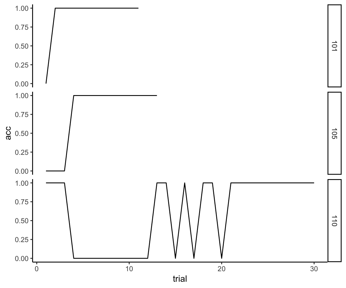
Now we still have the problem that there are a variable number of trials, so we need to generate an approximation of what the data would look like if all participants had been given the same number of trials.
6.2 Extrapolate individual curves until sample mean approaches asymptote
First, I’m going to make the very reasonable assumption that if a person has gotten 10 trials correct in a row, then, barring some kind of head trauma, they would have continued to get all subsequent trials correct. It’s just the nature of the task—once you acquire the rule you perform perfectly until the rule changes. So we extrapolate the unassessed trials like so:
max_trial <- max(reflective_examples$trial)
reflective_examples <- reflective_examples %>% group_by(sub) %>%
  complete(trial = 1:max_trial, fill = list(acc = 1)) %>%
  ungroup %>% arrange(sub, trial)
ggplot(reflective_examples, aes(x = trial, y = acc)) + facet_grid(sub~.) +
  theme_classic() +
  geom_line()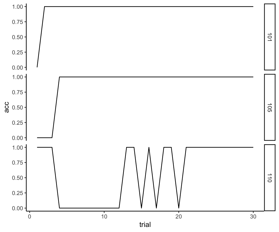
However, just extending out everyone’s learning curves to match the number of trials required by the slowest learner in the whole sample (which is 45) is probably not a good idea. If we look at the sample-wide distribution of the number of trials to reach criterion on the first rule, we see that it has an exceptionally long tail:
trials_to_criterion <- reflect_no_exclude %>%
  group_by(sub) %>%
  summarize(criterion = max(trial))
qplot(x = criterion, geom = "density", data = trials_to_criterion,
      adjust = 2, xlab = "Trials to Criterion") + theme_classic()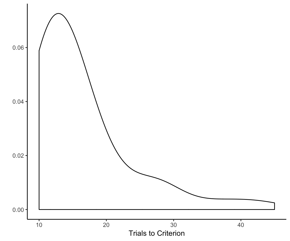
What we need to do is come up with a set number of trials that gives most, but not every single participant, sufficient time to learn the first rule but not so much time that we end up squashing outcome variability for a huge chunk of the reflective learning curve. (There’s no point in trying to analyze variance that does not exist.)
So what is the right number of trials? There are a number of ways that one might go about trying to determine this. Just eyeballing it, I’d say 15— that’s how many trials I’d give for the first rule if I were designing the experiment from scratch. But we probably want a criterion that does not rely on my subjective preference for multiples of 5. The sample mean might be a good choice—that would “mean” 16 trials. (Sorry for that.)
What I ultimately went with, though, was the 75th percentile of the number of trials needed to reach criterion. Why 75th?
To my mind, 75% corresponds best to the idea of “most but not all” because it is literally halfway between half and all. Note that, while the 75th percentile is an arbitrary choice, it’s not as arbitrary as say the 83.3rd percentile. Moreover, I am basing this decision on the 75th percentile of the entire sample, not the individual treatment conditions. This amounts to 19 trials based on the sample with excluded participants, and 18 trials for the sample that did not exclude participants.
I kind of doubt that there is much daylight between 15 and 19 trials in terms of the impact this choice has on the results, but I deliberately did not look into that so that this knowledge could not bias this choice. I simply committed to the 75th percentile and went with it, and I will leave it to the interested reader to see what would happen if another number of trials had been used.
trial_75th <- map(
  list(with_exclusions = reflect_with_exclude,
       without_exclusions = reflect_no_exclude),
  ~ unlist(
    group_by(.x, sub) %>% summarize(max_trial = max(trial)) %>% ungroup %>%
    summarize(upper_max_trial = ceiling(quantile(max_trial, .75)))))
trial_75th
## $with_exclusions
## upper_max_trial.75%
## 19
##
## $without_exclusions
## upper_max_trial.75%
## 18reflect_complete_no_exclude <- reflect_no_exclude %>%
filter(trial <= trial_75th$without_exclusions) %>%
group_by(sub, wt, tx, task, task_order, feature, condition) %>%
complete(trial = 1:trial_75th$without_exclusions,
fill = list(acc = 1)) %>%
ungroup %>% arrange(sub, trial) %>%
mutate(order = as.integer(task_order == "reflexive first"))
reflect_complete_with_exclude <- reflect_with_exclude %>%
filter(trial <= trial_75th$with_exclusions) %>%
group_by(sub, wt, tx, task, task_order, feature, condition) %>%
complete(trial = 1:trial_75th$with_exclusions,
fill = list(acc = 1)) %>%
ungroup %>% arrange(sub, trial) %>%
mutate(order = as.integer(task_order == "reflexive first"))Just as a sanity check, let’s plot the sample mean accuracy as a function of trial and see if it produces a reasonable-looking learning curve:
reflective_mean_curve <- reflect_complete_with_exclude %>%
  group_by(trial) %>%
  summarize(acc = mean(acc))
ggplot(reflective_mean_curve, aes(x = trial, y = acc)) +
  geom_line() + geom_smooth(method = "loess", se = F) + theme_classic() +
  coord_cartesian(ylim = c(.5, 1)) + ggtitle("Reflective Task")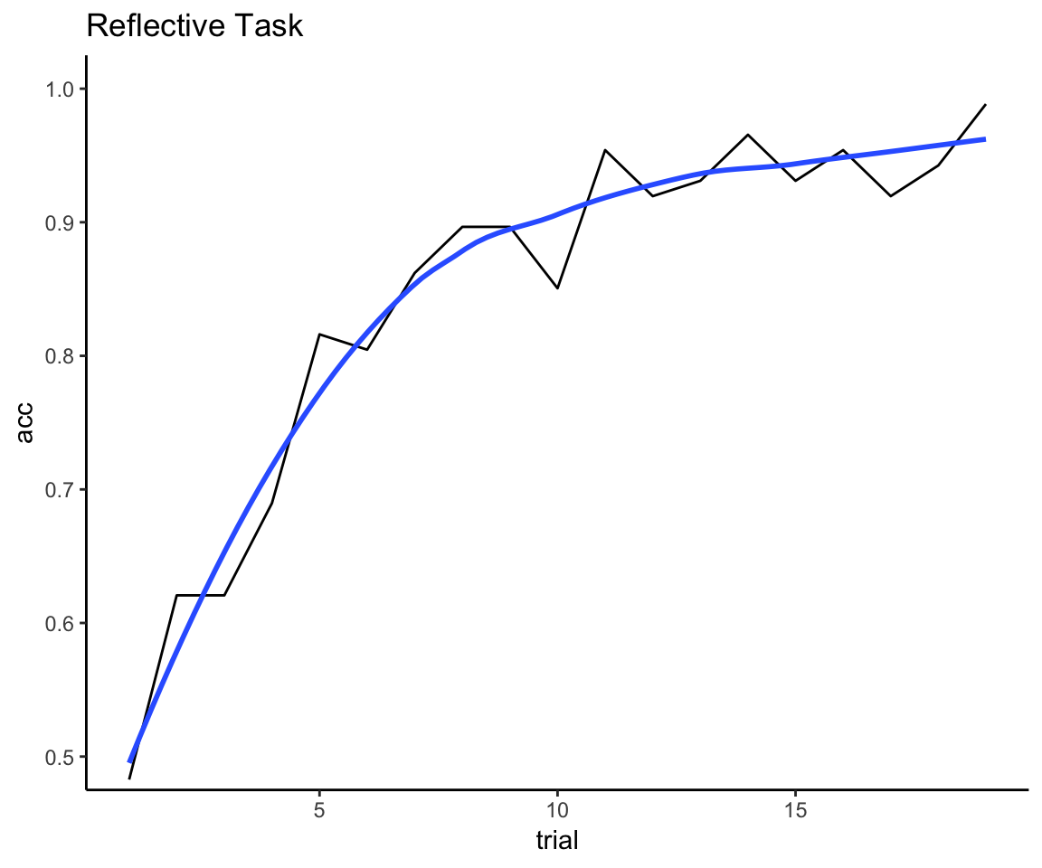
That looks about right to me: we have enough trials to see the mean curve deaccelerate, but not so many trials that we end up with 100% accuracy for everyone.
6.3 Scale trial number
We’re now close to having two learning curves that we can compare within person. But we still have to account for the fact that the reflexive task has 132 more trials than the reflective task and that a span of 18 trials in the reflexive task shows marginal improvement at best whereas it encompasses the entire learning curve for the reflective task.
This is the easiest problem to solve: just scale the value of trial so that the first trial is 0 and the last trial is 1. Rescaling covariates is standard practice anyway to facilitate convergence of a generalized linear mixed effects model (see next section), which needs all covariates to be at similar numerical scale. It also means that the beta coefficients for trial effects in the models will have a more interpretable meaning as the amount of improvement at the end of training relative to the start of training for both tasks.
reflect_complete_no_exclude <- reflect_complete_no_exclude %>%
  mutate(trial = (trial-1) / (max(trial) - 1))
reflect_complete_with_exclude <- reflect_complete_with_exclude %>%
  mutate(trial = (trial-1) / (max(trial) - 1))
reflex_no_exclude <- reflex_no_exclude %>%
  mutate(trial = (trial-1) / (max(trial) - 1))
reflex_with_exclude <- reflex_with_exclude %>%
  mutate(trial = (trial-1) / (max(trial) - 1))
all_data <- bind_rows(reflect_complete_no_exclude, reflex_no_exclude)
data_with_exclusions <- bind_rows(reflect_complete_with_exclude,
                                  reflex_with_exclude)
7 Statistical Analyses
7.1 Learning curve analysis
I’m starting with the analysis that is presented last in the paper because a) it’s the one that I did, and b) from my perspective it’s the primary analysis. That’s because I personally didn’t try or even consider any other analytic approach other than a generalized linear mixed effects regression (GLMER) with a binomial link function, given that the raw data consisted of time series of Bernoulli trials (each trial is either a success or failure). Here’s all the reasons why:
The model is fit to the raw measured values in their native Boolean form, so we don’t need to operationalize the measured values into some other construct (e.g., accuracy or trials to criterion).
It makes use of every single observation and explicitly models individual change across time within each task.
It does not need to have the same number of observations per cell, and time can be modeled as continuous rather than a fixed set of points. This is helpful given that we have defined one unit of time to contain 150 observations for the reflexive task and 18 observations for the reflective task.
The model is specified as follows:
A fixed intercept of 0. The logic for this is that the intercept coefficient represents the log odds of a correct response for the first trial (because we have coded that time point as 0), and we know that the odds of a correct response (for either group) on the first trial must be 50/50, i.e., the odds ratio is equal to 1, and the log of 1 is 0. Any observed departures from this must necessarily be noise unless we believe that acetaminophen grants psychic powers to know the right answer before getting any feedback. Therefore, the model should not try to fit an intercept different from 0.
An effect of trial. The probability of success should increase as a function of trial regardless of task or treatment condition.
An effect of trial that is conditional on learning task. The probability of success as a function of trial should increase faster for the reflective task than for the the reflexive task, regardless of treatment condition.
An effect of trial that is conditional on treatment. The probability of success as a function of trial should not change as a function of treatment independent of task. (Acetaminophen was hypothesized to push reflective learning up and reflexive learning down, but in a zero-sum fashion, i.e., no net gain or loss in overall learning ability.)
An effect of trial that is conditional on an effect of treatment that is conditional on task. The probability of success as a function of trial is hypothesized to increase faster for the acetaminophen group for the reflective task, and it should increase slower for the acetaminophen group for the reflexive task.
A random slope of trial for each participant in each task. This specifies that the trial-level observations are clustered within subject and within task.
7.1.1 With participant exclusions and without weighting adjustment (published analysis)
library(lme4)
omnibus_glm_orig <- glmer(acc ~ 0 + trial + trial:task + trial:tx +
                            trial:task:tx + ((0 + trial) | sub:task),
                          data = data_with_exclusions, family = "binomial")
summary(omnibus_glm_orig)
## Generalized linear mixed model fit by maximum likelihood (Laplace
## Approximation) [glmerMod]
## Family: binomial ( logit )
## Formula: acc ~ 0 + trial + trial:task + trial:tx + trial:task:tx + ((0 +
## trial) | sub:task)
## Data: data_with_exclusions
##
## AIC BIC logLik deviance df.resid
## 18200.8 18238.8 -9095.4 18190.8 14698
##
## Scaled residuals:
## Min 1Q Median 3Q Max
## -9.5039 -1.0555 0.5608 0.8631 1.1118
##
## Random effects:
## Groups Name Variance Std.Dev.
## sub:task trial 1.275 1.129
## Number of obs: 14703, groups: sub:task, 174
##
## Fixed effects:
## Estimate Std. Error z value Pr(>|z|)
## trial 1.1099 0.1735 6.396 1.60e-10 ***
## trial:task 2.7925 0.3531 7.908 2.61e-15 ***
## trial:tx -0.3252 0.2519 -1.291 0.197
## trial:task:tx 2.5333 0.5913 4.285 1.83e-05 ***
## ---
## Signif. codes: 0 '***' 0.001 '**' 0.01 '*' 0.05 '.' 0.1 ' ' 1
##
## Correlation of Fixed Effects:
## trial trl:ts trl:tx
## trial:task -0.478
## trial:tx -0.688 0.332
## tril:tsk:tx 0.290 -0.559 -0.424Not surprisingly we see strong effects for trial and the trial \(\times\) task interaction. The hypothesized trial \(\times\) task \(\times\) treatment interaction was also substantial.4 To interpret this interaction, we can use the effects package to plot the model of the learning curves that were fit, but I’m going to hold off on this until we have fit the new models.
7.1.2 With participant exclusions and weighting adjustment (new analysis)
omnibus_glm_new_with_excl <- glmer(acc ~ 0 + trial + trial:task + trial:tx +
                       trial:task:tx + ((0 + trial) | sub:task),
                       data = data_with_exclusions, family = "binomial",
                       weights = wt)
summary(omnibus_glm_new_with_excl)
## Generalized linear mixed model fit by maximum likelihood (Laplace
## Approximation) [glmerMod]
## Family: binomial ( logit )
## Formula: acc ~ 0 + trial + trial:task + trial:tx + trial:task:tx + ((0 +
## trial) | sub:task)
## Data: data_with_exclusions
## Weights: wt
##
## AIC BIC logLik deviance df.resid
## 18233.2 18271.1 -9111.6 18223.2 14698
##
## Scaled residuals:
## Min 1Q Median 3Q Max
## -9.2672 -1.0253 0.5499 0.8412 1.1311
##
## Random effects:
## Groups Name Variance Std.Dev.
## sub:task trial 1.295 1.138
## Number of obs: 14703, groups: sub:task, 174
##
## Fixed effects:
## Estimate Std. Error z value Pr(>|z|)
## trial 1.1080 0.1755 6.314 2.72e-10 ***
## trial:task 2.7330 0.3591 7.610 2.74e-14 ***
## trial:tx -0.3217 0.2540 -1.266 0.205
## trial:task:tx 2.5492 0.5830 4.373 1.23e-05 ***
## ---
## Signif. codes: 0 '***' 0.001 '**' 0.01 '*' 0.05 '.' 0.1 ' ' 1
##
## Correlation of Fixed Effects:
## trial trl:ts trl:tx
## trial:task -0.474
## trial:tx -0.690 0.329
## tril:tsk:tx 0.298 -0.571 -0.434The estimate of treatment effect does not change much and actually becomes marginally stronger when we use the correction weights (b = 2.55, up from b = 2.53).
7.1.3 With weighting adjustment and without participant exclusions (new analysis)
omnibus_glm_new <- glmer(acc ~ 0 + trial + trial:task + trial:tx +
                       trial:task:tx + ((0 + trial) | sub:task),
                       data = all_data, family = "binomial",
                       weights = wt)
summary(omnibus_glm_new)
## Generalized linear mixed model fit by maximum likelihood (Laplace
## Approximation) [glmerMod]
## Family: binomial ( logit )
## Formula: acc ~ 0 + trial + trial:task + trial:tx + trial:task:tx + ((0 +
## trial) | sub:task)
## Data: all_data
## Weights: wt
##
## AIC BIC logLik deviance df.resid
## 20755.4 20794.0 -10372.7 20745.4 16627
##
## Scaled residuals:
## Min 1Q Median 3Q Max
## -10.1211 -1.0252 0.5515 0.8493 1.2215
##
## Random effects:
## Groups Name Variance Std.Dev.
## sub:task trial 1.311 1.145
## Number of obs: 16632, groups: sub:task, 198
##
## Fixed effects:
## Estimate Std. Error z value Pr(>|z|)
## trial 1.0633 0.1688 6.299 3.01e-10 ***
## trial:task 2.7630 0.3461 7.983 1.42e-15 ***
## trial:tx -0.3420 0.2391 -1.430 0.153
## trial:task:tx 2.7184 0.5641 4.819 1.45e-06 ***
## ---
## Signif. codes: 0 '***' 0.001 '**' 0.01 '*' 0.05 '.' 0.1 ' ' 1
##
## Correlation of Fixed Effects:
## trial trl:ts trl:tx
## trial:task -0.474
## trial:tx -0.706 0.337
## tril:tsk:tx 0.296 -0.566 -0.422Note that when we use all available data the three-way interaction effect has a somewhat larger coefficient and its p-value is an order of magnitude smaller. Let’s now reproduce the plot of the learning curves from our paper, but this time using the full sample with the weighting adjustment to balance task order.
library(effects); library(grid); library(gridExtra)
omni_glm_eff <- allEffects(
    omnibus_glm_new,
     xlevels = list(trial = seq(0,1,.1),
                    task = c(0, 1),
                    tx = c(0, 1)
                    )
  )
plot_data <- omni_glm_eff$`trial:task:tx`$x
plot_data$p <- omni_glm_eff$`trial:task:tx`$fit %>% as.vector() %>%
  omni_glm_eff$`trial:task:tx`$transformation$inverse()
plot_data$lower <- omni_glm_eff$`trial:task:tx`$lower %>% as.vector() %>%
   omni_glm_eff$`trial:task:tx`$transformation$inverse()
plot_data$upper <- omni_glm_eff$`trial:task:tx`$upper %>% as.vector() %>%
   omni_glm_eff$`trial:task:tx`$transformation$inverse()
plot_data$task <- factor(plot_data$task,
                         labels = c("Reflexive-Optimal",
                                    "Reflective-Optimal"))
plot_data$tx <- factor(plot_data$tx,
                       labels = c("Placebo", "Acetaminophen"))
plot_data <- plot_data %>%
  mutate(trial = ifelse(task == "Reflexive-Optimal",
                        # descale back to trial number
                        trial*149+1, trial*18+1))
reflexive <- ggplot(data = plot_data %>% filter(task == "Reflexive-Optimal"),
                    aes(x = trial, y = p, color = tx, linetype = tx)) +
   theme_classic() +
  geom_line(size = 1) +
  geom_ribbon(aes(x = trial, ymin = lower, ymax = upper),
                            alpha = .1, color = NA) +
  facet_wrap(facets = ~ task) +
  coord_cartesian(ylim = c(.5, 1)) +
  labs(x = "", y = "") +
  theme(legend.title = element_blank(),
        legend.position = c(.2,.9),
        strip.text = element_text(size = 14),
        legend.text = element_text(size = 12),
        panel.grid.major = element_blank(),
        panel.grid.minor = element_blank(),
        axis.line = element_line(size = .5),
        axis.text.x = element_text(size = 12),
        axis.text.y = element_text(size = 12),
        axis.title.x = element_text(size = 14),
        axis.title.y = element_text(size = 14),
        strip.background = element_blank())
reflective <- ggplot(
  data = plot_data %>% filter(task == "Reflective-Optimal"),
  aes(x = trial, y = p, color = tx, linetype = tx)) +
   theme_classic() +
  geom_line(size = 1) +
  geom_ribbon(aes(x = trial, ymin = lower, ymax = upper),
              alpha = .1, color = NA) +
  facet_wrap(facets = ~ task) +
  coord_cartesian(ylim = c(.5, 1)) +
  labs(x = "", y = "") +
  theme(legend.position = "none",
        strip.text = element_text(size = 14),
        panel.grid.major = element_blank(),
        panel.grid.minor = element_blank(),
        axis.line = element_line(size = .5),
        axis.text.x = element_text(size = 12),
        axis.text.y = element_text(size = 12),
        axis.title.x = element_text(size = 14),
        axis.title.y = element_text(size = 14),
        strip.background = element_blank())
final_plot <- arrangeGrob(
  reflexive, reflective, nrow = 1, ncol = 2,
  left = textGrob("Probability of correct response",
                  rot = 90,
                  gp=gpar(fontsize = 12)),
  bottom = textGrob("Trial number", gp=gpar(fontsize = 12))
  )
plot(final_plot)
The three-way interaction reflects that the difference between the acetaminophen group and the placebo group shifts an improbable amount between the reflexive and reflective tasks (if the difference between acetaminophen and placebo learning curves really does not depend on task), and the direction of the difference reverses as the COVIS model would predict. There is a great deal more uncertainty in forecasting the probability of success on the reflexive task, whereas the confidence intervals around the predictions of reflective task performance are relatively narrow.
Everyone always wants to follow up on the finding of an interesting interaction with some statement about whether there is a “significant difference” within each group. I’m not a fan of this unless a pure between-group difference was hypothesized in advance and the study was powered to detect it. Power gets a significant boost here from the fact that the contrast between tasks is happening within, not between, subjects, which is lost the moment we start fitting “follow-up” models within each task separately. So, rather than fit additional models to address the question of the “simple effect” of acetaminophen within task, I used the same model above to construct odds ratios (acetaminophen / placebo) from the predicted probabilities and their confidence intervals for time points of interest within each task: final trial of the reflexive task (trial = 150) and minimum trial to reach criterion in the reflective task (trial = 10).
plot_data %>% filter(task == "Reflective-Optimal", trial == 10) %>%
  group_by(task) %>%
  summarize(OR = p[2]/p[1],
            low = lower[2]/upper[1],
            high = upper[2]/lower[1]) %>%
  bind_rows(
    plot_data %>% filter(task == "Reflexive-Optimal", trial == 150) %>%
      group_by(task) %>%
      summarize(OR = p[2]/p[1],
            low = lower[2]/upper[1],
            high = upper[2]/lower[1])
  )
## # A tibble: 2 x 4
## task OR low high
## <fct> <dbl> <dbl> <dbl>
## 1 Reflective-Optimal 1.10 1.04 1.16
## 2 Reflexive-Optimal 0.905 0.744 1.10So the acetaminophen-treated group showed less than a 10% improvement on the reflective task and less than a 10% worsening on the reflexive task, with a 95% confidence interval for reflexive that includes no difference. In other words, the effect of acetaminophen on either learning curve alone was relatively small. But the small effects are in opposite directions, which adds up to a larger interaction effect.
7.1.4 Analogous model of task order effect
One final thing I’m curious about. What sort of order effect is there anyway, independent of treatment effect? To fit this, we just swap tx for order in the above model. For expedience, I am only going to fit this to the full data set (no exclusions) using the counterbalancing weights.
omnibus_glm_order <- glmer(acc ~ 0 + trial + trial:task + trial:order +
                       trial:task:order + ((0 + trial) | sub:task),
                       data = all_data, family = "binomial",
                       weights = wt)
summary(omnibus_glm_order)
## Generalized linear mixed model fit by maximum likelihood (Laplace
## Approximation) [glmerMod]
## Family: binomial ( logit )
## Formula: acc ~ 0 + trial + trial:task + trial:order + trial:task:order +
## ((0 + trial) | sub:task)
## Data: all_data
## Weights: wt
##
## AIC BIC logLik deviance df.resid
## 20777.1 20815.7 -10383.6 20767.1 16627
##
## Scaled residuals:
## Min 1Q Median 3Q Max
## -7.3963 -1.0234 0.5513 0.8506 1.2201
##
## Random effects:
## Groups Name Variance Std.Dev.
## sub:task trial 1.714 1.309
## Number of obs: 16632, groups: sub:task, 198
##
## Fixed effects:
## Estimate Std. Error z value Pr(>|z|)
## trial 1.4071 0.4270 3.295 0.000984 ***
## trial:task 3.4035 0.5675 5.997 2.01e-09 ***
## trial:order -0.3401 0.2706 -1.257 0.208814
## trial:task:order 0.4869 0.5558 0.876 0.381004
## ---
## Signif. codes: 0 '***' 0.001 '**' 0.01 '*' 0.05 '.' 0.1 ' ' 1
##
## Correlation of Fixed Effects:
## trial trl:ts trl:rd
## trial:task -0.749
## trial:order -0.948 0.712
## trl:tsk:rdr 0.461 -0.732 -0.486
Fortunately, there does not seem to be much of an effect of order on the learning curves, which explains why the results do not change much when adjusted for the task-order imbalance.
7.1.5 Conclusion
The results are certainly consistent with what my co-authors expected would happen if acetaminophen boosted serotonin signaling. And the results were unaltered after using adjustment weights to correct for the counterbalancing problem and only strengthened by including all available data. That of course does not prove that acetaminophen did boost serotonin signaling, or that this is the only possible explanation for what was found. Moreover, sampling error is a real thing, and this finding could always just be a fluke of this particular sample.
It is important to acknowledge that we had to compute “as if” approximations for the reflective learning curves in order to compare them to the reflexive learning curves,5 but I don’t know how else to make the analysis work. You’re about to see some other things that my co-authors tried, but solving one problem invariably leads to another.
For example, counting trials to criterion eliminates the problem of needing to extrapolate or discard any data for the reflective task, but it introduces the problem that the majority of the sample never reached criterion on the reflexive task—which means we can’t compare trials to criterion between tasks unless we assign an arbitrary maximum count to more than half the sample for the reflexive task. The customary practice in this scenario is to assign the maximum number of trials (or that number + 1), so we assigned the majority of participants who did not reach criterion a value of 150. But obviously this does not mean that these participants actually did reach criterion after 150 trials, and there is no way for us to know how many more trials each person would have needed. We only know that, for the majority of the sample, the true number is beyond the 150 trials that we measured—a classic ceiling effect.
Bottom line, there’s no slam-dunk solution, save using a different reflective task where learning is slow and incremental (which, despite extensive effort, the authors were unable to develop). This is why it is a good idea to look at the data in a few different ways and take all evidence into account when forming conclusions, which is what we tried to do in our article.
I now turn to reproducing the analyses that I did not personally contribute to the manuscript.
7.2 Overall accuracy
The first analysis presented in the article compared the mean accuracy across all 150 trials of both tasks. The problem this analysis solves is that it equates the number of observations per task. (In the previous learning curve analysis, the reflexive task has ~8 times as many observations as the reflective task; in the subsequent trials-to-criterion analysis, 100% of the sample reached criterion for the reflective task, but for the reflexive task, criterion was only observed for 38% of the sample.) The problem this analysis creates is that mean accuracy across all trials is not a measure of learning. Let me explain why.
There are two basic features of interest when we look at acquisition data from a learning task: the amount of acquisition (how much was learned by the end of training?) and the rate of acquisition (how quickly was the task acquired?). To assess amount, one should look at the final trial or average the last block of trials; that’s not a useful thing to look at here since everyone in the reflective task is trained to the point of mastery. The standard way of assessing rate is to construct a statistical model of change over time (as I did in the previous analysis) or, for tasks with a predefined criterion of mastery, look at the time needed to achieve mastery (as I will do in the next analysis).
Both of these approaches, but not mean accuracy, were used in the previous study that the acetaminophen study was based on. I point this out because I think it is important when evaluating the evidence to keep in mind that two of the analyses—trials to criterion and learning rate—have established precedent, and one—overall accuracy—is being introduced for the first time. This is evident if you’ve followed this group’s work on this topic, but we neglected to point this out in the manuscript.
As a general policy, I would only recommend averaging over trials when the assumption of exchangeability is met, i.e., any one trial gives you the same information as any other. This is true for almost all of the psychometric tasks used by this lab group (e.g., measures of attention bias), which I think is what led them to average across all trials here: they’re accustomed to doing this for all their other tasks which do not have a learning component.6 But trials in a learning experiment are by definition non-exchangeable: for example, the first trial does not give you the same information as the last trial.
So the mean of all 150 trials—what is it telling us? For the reflexive task, I’d say it’s a proxy for learning rate. Participants who acquire the task faster will end up with more accurate trials and therefore a higher mean accuracy overall. For the reflective task, if there had been a fixed number of rules and a fixed number of trials per rule, I’d say that it was also a proxy of learning rate. But let’s think through the consequences of having given a variable number of rules/trials conditional on individual performance.
First, let’s say we’re just comparing one rule, the first one. And let’s say we’re comparing two learners. One is fast and meets criterion after 12 trials:
fast_learner <- tibble(
  trial = 1:12,
  accuracy = c(0,0, rep(1,10)),
  id = "fast learner"
)
The other is slow and meets the criterion after 24 trials:
slow_learner <- tibble(
  trial = 1:24,
  accuracy = c(0,1,1,1,1,0,1,1,0,1,1,1,1,0, rep(1, 10)),
  id = "slow learner"
)
But, as you can see, despite the fact that one person learned the rule in half the time as the other…
learners <- bind_rows(fast_learner, slow_learner)
ggplot(learners, aes(x = trial, y = accuracy)) + facet_wrap(~ id) +
  geom_line() +
  theme_classic() +
  scale_x_continuous(breaks = seq(2, 24, by = 2)) +
  theme(legend.title = element_blank(),
        legend.position = c(.9,.1)) +
  coord_cartesian(ylim = c(0,1))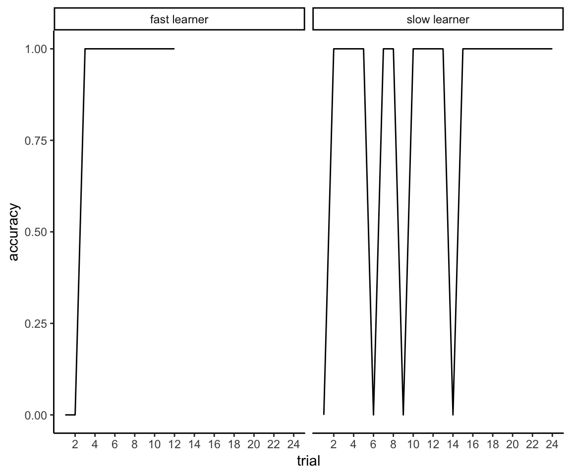
they have the exact same mean accuracy:
learners %>% group_by(id) %>% summarize(mean_accuracy = mean(accuracy))## # A tibble: 2 x 2
## id mean_accuracy
## <chr> <dbl>
## 1 fast learner 0.833
## 2 slow learner 0.833You could even come up with scenarios where the slow learner has a higher mean accuracy than the fast learner.
The same problem extends to all 150 trials. Here’s a fast learner who masters 6 rules over the course of the experiment:
fast_learner <- tibble(
  id = "fast learner",
  trial = 1:150,
  accuracy = rep(c(rep(c(0,1,0),times = 5), rep(1,10)), times = 6),
  rule = factor(rep(1:6, each = 150/6))
)
Here’s a slow learner who only masters 3 rules over the course of the experiment:
slow_learner <- tibble(
   id = "slow learner",
  trial = 1:150,
  accuracy = rep(c(rep(c(1,0,1,0), times = 10), rep(1,10)), times = 3),
  rule = factor(rep(1:3, each = 150/3), levels = 1:6)
)
And here’s their mean accuracy across all 150 trials:
learners <- bind_rows(fast_learner, slow_learner)
learners %>% group_by(id) %>% summarize(mean_accuracy = mean(accuracy))
## # A tibble: 2 x 2
## id mean_accuracy
## <chr> <dbl>
## 1 fast learner 0.6
## 2 slow learner 0.6Despite the fact one learner is obviously twice as good as the other:
ggplot(learners, aes(x = trial, y = accuracy, color = rule)) +
  facet_grid(id ~.) + ggtitle("Reflective Task") +
  geom_smooth(method = "loess", se = FALSE) + theme_classic() +
  coord_cartesian(ylim = c(0,1))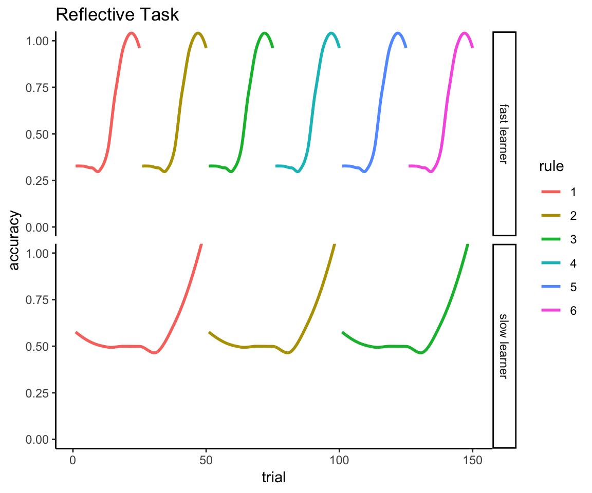
You see the problem.
The way this gets reported in our published manuscript is that the following analysis is reported first as “confirmatory” because this is what my co-authors had planned to run and in fact had already run before I pointed out the above psychometric problems:
7.2.1 Accuracy of all trials
7.2.1.1 With participant exclusions and without weighting adjustment (published analysis)
library(ez)
accuracy_data <- bind_rows(reflexive_task, reflective_task) %>%
  mutate(task = factor(task, labels = c("reflexive", "reflective")),
         tx = factor(tx, labels = c("placebo", "acetaminophen"))) %>%
  group_by(sub, task, tx) %>%
  summarize(Meanacc = mean(acc)) %>%
  ungroup()
accuracy_with_exclude <- accuracy_data %>%
  filter(!sub %in% to_exclude) %>%
  mutate(sub = fct_drop(sub)) %>%
  left_join(design_with_exclude %>% select(-tx), by = "sub")
accuracy_data <- accuracy_data %>%
  left_join(design_no_exclude %>% select(-tx), by = "sub")
accuracyanova <- ezANOVA(
  data = accuracy_with_exclude,
  dv = Meanacc, wid = sub, within = task, between = tx, type=3,
  detailed = TRUE
)
print(accuracyanova, digits = 3)
## $ANOVA
## Effect DFn DFd SSn SSd F p p<.05 ges
## 1 (Intercept) 1 85 6.87e+01 0.546 1.07e+04 3.45e-91 * 0.983988
## 2 tx 1 85 2.29e-04 0.546 3.56e-02 8.51e-01 0.000204
## 3 task 1 85 5.97e-03 0.572 8.87e-01 3.49e-01 0.005315
## 4 tx:task 1 85 2.27e-02 0.572 3.38e+00 6.97e-02 0.019929Note that the last column on the right, ges, is the generalized eta-squared, which is the effect size estimate reported in our publication. Please be aware that generalized eta-squared is NOT the same as partial eta-squared!
7.2.1.2 With participant exclusions and weighting adjustment (new analysis)
So the ANOVA function does not support the use of observation weights, but here’s a fun fact: in the special case of a single within-subject factor with only two levels, the treatment \(\times\) task interaction is equivalent to a linear model of treatment predicting the within-subject difference between tasks.
accuracy_data <- accuracy_data %>% group_by(sub, tx, wt, task_order) %>%
  summarize(reflect_reflex_diff = Meanacc[task == "reflective"] -
              Meanacc[task == "reflexive"])
accuracy_with_exclude <- accuracy_with_exclude %>%
  group_by(sub, tx, wt, task_order) %>%
  summarize(reflect_reflex_diff = Meanacc[task == "reflective"] -
              Meanacc[task == "reflexive"])
accuracy_lm <- lm(reflect_reflex_diff ~ tx, data = accuracy_with_exclude)
summary(accuracy_lm)
##
## Call:
## lm(formula = reflect_reflex_diff ~ tx, data = accuracy_with_exclude)
##
## Residuals:
## Min 1Q Median 3Q Max
## -0.32130 -0.09507 0.01783 0.09116 0.24449
##
## Coefficients:
## Estimate Std. Error t value Pr(>|t|)
## (Intercept) -0.01116 0.01711 -0.652 0.5160
## txacetaminophen 0.04579 0.02492 1.837 0.0697 .
## ---
## Signif. codes: 0 '***' 0.001 '**' 0.01 '*' 0.05 '.' 0.1 ' ' 1
##
## Residual standard error: 0.116 on 85 degrees of freedom
## Multiple R-squared: 0.0382, Adjusted R-squared: 0.02688
## F-statistic: 3.376 on 1 and 85 DF, p-value: 0.06965Note that the p-value for the acetaminophen effect in this model, .0697, is identical to the p-value for the interaction effect in the preceding ANOVA. So now we can see how this p-value changes when we add the weighting adjustment.
accuracy_lm <- lm(reflect_reflex_diff ~ tx, data = accuracy_with_exclude,
                  weights = wt)
summary(accuracy_lm)
##
## Call:
## lm(formula = reflect_reflex_diff ~ tx, data = accuracy_with_exclude,
## weights = wt)
##
## Weighted Residuals:
## Min 1Q Median 3Q Max
## -0.30373 -0.09336 0.01359 0.07887 0.26097
##
## Coefficients:
## Estimate Std. Error t value Pr(>|t|)
## (Intercept) -0.004074 0.017781 -0.229 0.819
## txacetaminophen 0.036460 0.025146 1.450 0.151
##
## Residual standard error: 0.1173 on 85 degrees of freedom
## Multiple R-squared: 0.02414, Adjusted R-squared: 0.01266
## F-statistic: 2.102 on 1 and 85 DF, p-value: 0.15087.2.1.3 With weighting adjustment and without participant exclusions (new analysis)
accuracy_lm <- lm(reflect_reflex_diff ~ tx, data = accuracy_data, weights = wt)
summary(accuracy_lm)
##
## Call:
## lm(formula = reflect_reflex_diff ~ tx, data = accuracy_data,
## weights = wt)
##
## Weighted Residuals:
## Min 1Q Median 3Q Max
## -0.29022 -0.09322 0.01772 0.07683 0.26000
##
## Coefficients:
## Estimate Std. Error t value Pr(>|t|)
## (Intercept) -0.0003889 0.0163835 -0.024 0.981
## txacetaminophen 0.0278774 0.0231698 1.203 0.232
##
## Residual standard error: 0.1153 on 97 degrees of freedom
## Multiple R-squared: 0.0147, Adjusted R-squared: 0.004547
## F-statistic: 1.448 on 1 and 97 DF, p-value: 0.2318So that’s p = 0.07 for the treatment \(\times\) task interaction with exclusions and no weighting, p = 0.15 with exclusions and weighting, and p = 0.23 with weighting and no exclusions. So this measure clearly is picking up on order effects:
accuracy_lm <- lm(reflect_reflex_diff ~ task_order,
                  data = accuracy_data, weights = wt)
summary(accuracy_lm)
##
## Call:
## lm(formula = reflect_reflex_diff ~ task_order, data = accuracy_data,
## weights = wt)
##
## Weighted Residuals:
## Min 1Q Median 3Q Max
## -0.298538 -0.091260 0.009403 0.082899 0.247763
##
## Coefficients:
## Estimate Std. Error t value Pr(>|t|)
## (Intercept) 0.03649 0.01617 2.256 0.0263 *
## task_orderreflexive first -0.04588 0.02287 -2.006 0.0477 *
## ---
## Signif. codes: 0 '***' 0.001 '**' 0.01 '*' 0.05 '.' 0.1 ' ' 1
##
## Residual standard error: 0.1138 on 97 degrees of freedom
## Multiple R-squared: 0.03982, Adjusted R-squared: 0.02993
## F-statistic: 4.023 on 1 and 97 DF, p-value: 0.04766As one might expect, people tend to do better across the entire reflective task if they do it first.
ggplot(accuracy_data, aes(x = task_order, y = reflect_reflex_diff)) +
  theme_classic() +
  geom_boxplot() +
  ylab("Difference in task accuracy (reflective - reflexive)") +
  xlab("")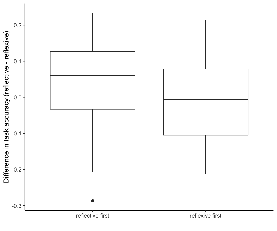
But how could one possibly use this analysis to draw conclusions about learning effects, given that a good learner can have the exact same overall accuracy as a poor learner? We put it this way in our manuscript:
Recall that in the reflective-optimal condition, rule changes occurred after 10 consecutive correct responses. The timing of when the rule changes occurred were not uniform across participants, which means that some participants had to learn more rule changes than others. This could suppress overall task accuracy. Therefore, an exploratory analysis was conducted to examine accuracy until the first rule change in the reflective condition.
That’s an accurate and concise description of the problem, and here’s the “exploratory” solution:
7.2.2 Accuracy using only the first rule
7.2.2.1 With participant exclusions and without weighting adjustment (published analysis)
accuracy_with_exclude <- data_with_exclusions %>%
  group_by(sub, task, tx, wt) %>%
  summarize(Meanacc = mean(acc)) %>%
  ungroup() %>%
  mutate(task = factor(task, labels = c("reflexive", "reflective")),
         tx = factor(tx, labels = c("placebo", "acetaminophen")),
         sub = fct_drop(sub))
accuracyanova <- ezANOVA(
  data = accuracy_with_exclude,
  dv = Meanacc, wid = unique(sub), within = .(task), between = tx, type=3,
  detailed = TRUE
)
print(accuracyanova, digits = 3)
## $ANOVA
## Effect DFn DFd SSn SSd F p p<.05 ges
## 1 (Intercept) 1 85 93.6502 1.10 7208.642 5.80e-84 * 0.97606
## 2 tx 1 85 0.0121 1.10 0.928 3.38e-01 0.00522
## 3 task 1 85 2.1506 1.19 153.232 1.02e-20 * 0.48352
## 4 tx:task 1 85 0.0760 1.19 5.416 2.23e-02 * 0.03203Once again, let’s just do a sanity check that a linear model of the accuracy difference gives the same result as the interaction effect:
accuracy_with_exclude <- accuracy_with_exclude %>%
  group_by(sub, tx, wt) %>%
  summarize(reflect_reflex_diff = Meanacc[task == "reflective"] -
              Meanacc[task == "reflexive"])
accuracy_lm <- lm(reflect_reflex_diff ~ tx, data = accuracy_with_exclude)
summary(accuracy_lm)
##
## Call:
## lm(formula = reflect_reflex_diff ~ tx, data = accuracy_with_exclude)
##
## Residuals:
## Min 1Q Median 3Q Max
## -0.55313 -0.10476 0.03611 0.12576 0.25915
##
## Coefficients:
## Estimate Std. Error t value Pr(>|t|)
## (Intercept) 0.18085 0.02470 7.321 1.29e-10 ***
## txacetaminophen 0.08374 0.03598 2.327 0.0223 *
## ---
## Signif. codes: 0 '***' 0.001 '**' 0.01 '*' 0.05 '.' 0.1 ' ' 1
##
## Residual standard error: 0.1675 on 85 degrees of freedom
## Multiple R-squared: 0.0599, Adjusted R-squared: 0.04884
## F-statistic: 5.416 on 1 and 85 DF, p-value: 0.022337.2.2.2 With participant exclusions and weighting adjustment (new analysis)
accuracy_lm <- lm(reflect_reflex_diff ~ tx, data = accuracy_with_exclude,
                  weights = wt)
summary(accuracy_lm)
##
## Call:
## lm(formula = reflect_reflex_diff ~ tx, data = accuracy_with_exclude,
## weights = wt)
##
## Weighted Residuals:
## Min 1Q Median 3Q Max
## -0.53236 -0.10233 0.04373 0.13012 0.28417
##
## Coefficients:
## Estimate Std. Error t value Pr(>|t|)
## (Intercept) 0.17482 0.02520 6.936 7.41e-10 ***
## txacetaminophen 0.08722 0.03564 2.447 0.0165 *
## ---
## Signif. codes: 0 '***' 0.001 '**' 0.01 '*' 0.05 '.' 0.1 ' ' 1
##
## Residual standard error: 0.1662 on 85 degrees of freedom
## Multiple R-squared: 0.0658, Adjusted R-squared: 0.05481
## F-statistic: 5.987 on 1 and 85 DF, p-value: 0.016477.2.2.3 With weighting adjustment and without participant exclusions (new analysis)
accuracy_data <- all_data %>%
  group_by(sub, task, tx, wt) %>%
  summarize(Meanacc = mean(acc)) %>%
  ungroup() %>%
  mutate(task = factor(task, labels = c("reflexive", "reflective")),
         tx = factor(tx, labels = c("placebo", "acetaminophen"))) %>%
  group_by(sub, tx, wt) %>%
  summarize(reflect_reflex_diff = Meanacc[task == "reflective"] -
              Meanacc[task == "reflexive"])
accuracy_lm <- lm(reflect_reflex_diff ~ tx, data = accuracy_data,
                  weights = wt)
summary(accuracy_lm)
##
## Call:
## lm(formula = reflect_reflex_diff ~ tx, data = accuracy_data,
## weights = wt)
##
## Weighted Residuals:
## Min 1Q Median 3Q Max
## -0.53160 -0.10162 0.03797 0.12327 0.29507
##
## Coefficients:
## Estimate Std. Error t value Pr(>|t|)
## (Intercept) 0.18009 0.02470 7.29 8.38e-11 ***
## txacetaminophen 0.10133 0.03494 2.90 0.00461 **
## ---
## Signif. codes: 0 '***' 0.001 '**' 0.01 '*' 0.05 '.' 0.1 ' ' 1
##
## Residual standard error: 0.1738 on 97 degrees of freedom
## Multiple R-squared: 0.0798, Adjusted R-squared: 0.07031
## F-statistic: 8.412 on 1 and 97 DF, p-value: 0.004612So that’s p = 0.02 for the treatment \(\times\) task interaction with exclusions and no weighting, p = 0.02 with exclusions and weighting, and p = 0.005 with weighting and no exclusions.
The confirmatory/exploratory labels that we attached to these two analyses raise a bit of a conundrum. On the one hand, it is certainly correct that my co-authors had originally planned to do the “confirmatory” analysis and only did the “exploratory” analysis once I pointed out the problems with the former. On the other hand, what about when a “confirmatory” analysis is discovered to have a serious flaw? Then it wouldn’t seem to “confirm” anything. And what if the “exploratory” analysis only seeks to correct that flaw? In this special case, isn’t the “exploratory” analysis a better test of the original hypothesis than the “confirmatory” analysis?
Points to ponder.
7.3 Trials to criterion
Another way to operationalize acquisition speed is to count the number of trials to criterion, which was predefined as 10 consecutive correct responses. You don’t have to take our word that it was predefined. The same criterion was used in previous work. And if you look in the reflective data file you can see that the rules were programmed to switch every time the person achieves 10 consecutive trials. (See the count.n variable.) Given that more than half the sample failed to meet criterion on the reflexive task, we need to assign a ceiling value to these cases, which we chose to be the maximum number of trials (150).
reflexive_criterion <- reflexive_data %>%
  group_by(sub, bottle) %>%
  summarize(criterion = if(10 %in% count.n){
    min(trial[count.n == 10])
  } else 150
  ) %>%
  ungroup() %>%
  mutate(task = "reflexive")
reflective_criterion <- reflective_data %>%
  group_by(sub, bottle) %>%
  summarize(criterion = if(10 %in% count.n){
    min(trial[count.n == 10])
  } else 150
  ) %>%
  ungroup() %>%
  mutate(task = "reflective")
criterion_all <- bind_rows(reflexive_criterion, reflective_criterion) %>%
  mutate(tx = factor(bottle, levels = c("placebo", "active"),
                     labels = c("Placebo", "Acetaminophen")),
         task = factor(task))
criterion_with_exclude <- criterion_all %>%
  filter(!sub %in% unlist(to_exclude)) %>%
  left_join(design_with_exclude %>% select(-tx), by = "sub") %>%
  mutate(sub = fct_drop(sub))
criterion_all <- criterion_all %>%
  left_join(design_no_exclude %>% select(-tx), by = "sub")
7.3.1 Task \(\times\) treatment ANOVA (published analysis)
crit.anova <- ezANOVA(data = criterion_with_exclude, dv = criterion,
                      wid = unique(sub), within = .(task),
                      between = .(tx), type=3, detailed = TRUE)
print(crit.anova, digits = 3)
## $ANOVA
## Effect DFn DFd SSn SSd F p p<.05 ges
## 1 (Intercept) 1 85 885328 61408 1225.45 2.88e-52 * 0.87082
## 2 tx 1 85 774 61408 1.07 3.04e-01 0.00586
## 3 task 1 85 517899 69921 629.58 4.63e-41 * 0.79771
## 4 tx:task 1 85 2998 69921 3.64 5.96e-02 0.02232Given the problems with this ANOVA (see next section), I am not bothering to redo this analysis with weights and without exclusions; this will instead be done for the more statistically valid within-task comparisons.
7.3.2 Problems with using an ANOVA for this measure
In our manuscript, we implied a potential problem with the results of this ANOVA, which is that “the majority of participants failed to reach criterion in the reflexive-optimal condition”. This led to “an exploratory analysis…to examine the influence of acetaminophen on reaching criterion (yes vs no) in the reflexive condition.”
I want to make this problem a bit more concrete and explain why we should be skeptical of the ANOVA results and why it is necessary to follow up with alternative models that are better suited to the distribution of the data.
First, trials-to-criterion is a count variable, but we’re treating it like a continuous variable when we run the ANOVA. Is that appropriate?
Here’s what the distribution of counts looks like for the reflective task:
ggplot(criterion_all %>% filter(task == "reflective"),
       aes(x = criterion, color = tx)) +
  geom_density(adjust = 2) + theme_classic() +
  xlab("Trials to Criterion") +
  theme(legend.title = element_blank(),
        legend.position = c(.8,.8)) +
  ggtitle("Reflective Task")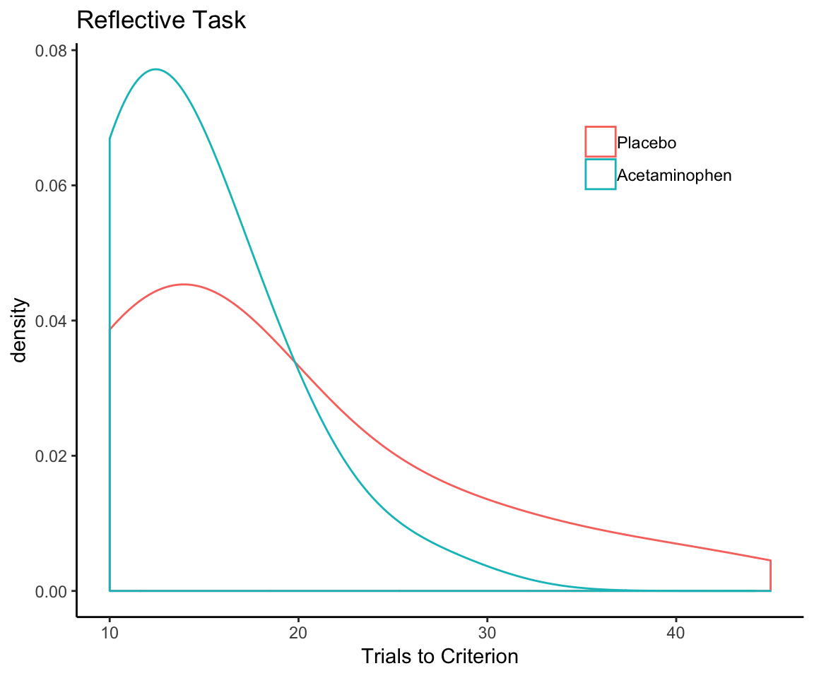
And here’s what it looks like for the reflexive task:
ggplot(criterion_all %>% filter(task == "reflexive"),
       aes(x = criterion, color = tx)) +
  geom_density(adjust = 2) + theme_classic() +
  xlab("Trials to Criterion") +
  theme(legend.title = element_blank(),
        legend.position = c(.8,.8)) +
  ggtitle("Reflexive Task")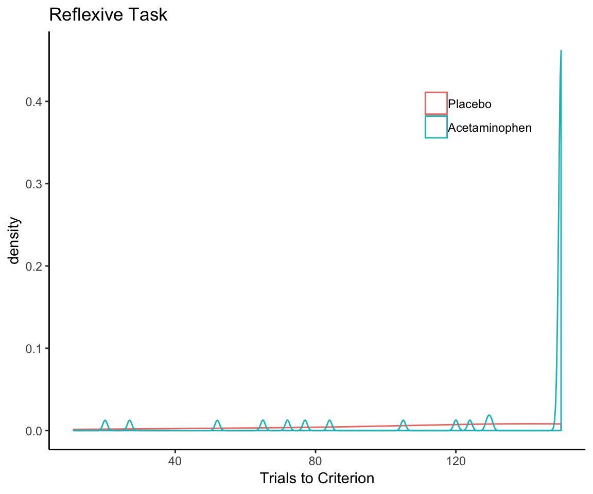
That makes me question whether it’s appropriate to be comparing the two tasks in terms of trials-to-criterion counts in the first place—not when 100% of one sample reaches the criterion on one task and only 38% of the sample reaches the criterion on the other. I think the best we can do here is a within-task comparison, in which we use different models appropriate to those different distributions.
7.3.3 Within-task comparisons of treatment effect
The lead author (RP) chose to use a Welch’s t-test to compare acetaminophen to placebo within the reflective task and, within the reflexive task, a chi-square test for the independence of treatment condition and meeting criterion.
If it were my analysis, I would have taken a different approach—not because there is anything wrong with RP’s approach, but because I prefer to stick to the GLM framework in general. It is furthermore necessary to use the GLM approach here so that we can use prior weights to correct for the task-order imbalance. As before, I will report the result I get using the previous data exclusions (with and without weighting) as well as all available data.
7.3.3.1 Reflective task
First, the trials-to-criterion for the reflective task looks like a count distribution, so let’s model it as such using a negative binomial GLM. Since count models assume a minimum possible count of 0 and the minimum possible count here is 10 (the criterion), we need to subtract a constant of 10 from the count in the model formula.
7.3.3.1.1 With participant exclusions and without weighting adjustment
MASS::glm.nb(
  criterion - 10 ~ tx,
  data = criterion_with_exclude %>% filter(task == "reflective")
) %>% summary
##
## Call:
## MASS::glm.nb(formula = criterion - 10 ~ tx, data = criterion_with_exclude %>%
## filter(task == "reflective"), init.theta = 1.072071181, link = log)
##
## Deviance Residuals:
## Min 1Q Median 3Q Max
## -2.1842 -1.0802 -0.3940 0.3975 1.7680
##
## Coefficients:
## Estimate Std. Error z value Pr(>|z|)
## (Intercept) 2.1802 0.1508 14.459 < 2e-16 ***
## txAcetaminophen -0.6207 0.2250 -2.759 0.00579 **
## ---
## Signif. codes: 0 '***' 0.001 '**' 0.01 '*' 0.05 '.' 0.1 ' ' 1
##
## (Dispersion parameter for Negative Binomial(1.0721) family taken to be 1)
##
## Null deviance: 105.777 on 86 degrees of freedom
## Residual deviance: 98.291 on 85 degrees of freedom
## AIC: 521.39
##
## Number of Fisher Scoring iterations: 1
##
##
## Theta: 1.072
## Std. Err.: 0.193
##
## 2 x log-likelihood: -515.3867.3.3.1.2 With participant exclusions and weighting adjustment
MASS::glm.nb(
  criterion - 10 ~ tx,
  data = criterion_with_exclude %>% filter(task == "reflective"),
  weights = wt
) %>% summary
##
## Call:
## MASS::glm.nb(formula = criterion - 10 ~ tx, data = criterion_with_exclude %>%
## filter(task == "reflective"), weights = wt, init.theta = 1.066677898,
## link = log)
##
## Deviance Residuals:
## Min 1Q Median 3Q Max
## -2.4187 -1.0108 -0.4647 0.4150 1.8612
##
## Coefficients:
## Estimate Std. Error z value Pr(>|z|)
## (Intercept) 2.2248 0.1550 14.35 < 2e-16 ***
## txAcetaminophen -0.6437 0.2243 -2.87 0.00411 **
## ---
## Signif. codes: 0 '***' 0.001 '**' 0.01 '*' 0.05 '.' 0.1 ' ' 1
##
## (Dispersion parameter for Negative Binomial(1.0667) family taken to be 1)
##
## Null deviance: 106.292 on 86 degrees of freedom
## Residual deviance: 98.134 on 85 degrees of freedom
## AIC: 523.92
##
## Number of Fisher Scoring iterations: 1
##
##
## Theta: 1.067
## Std. Err.: 0.191
##
## 2 x log-likelihood: -517.9207.3.3.1.3 With weighting adjustment and without participant exclusions
MASS::glm.nb(
  criterion - 10 ~ tx,
  data = criterion_all %>% filter(task == "reflective"),
  weights = wt
) %>% summary
##
## Call:
## MASS::glm.nb(formula = criterion - 10 ~ tx, data = criterion_all %>%
## filter(task == "reflective"), weights = wt, init.theta = 0.9601380881,
## link = log)
##
## Deviance Residuals:
## Min 1Q Median 3Q Max
## -2.3458 -0.9429 -0.4292 0.4090 1.9235
##
## Coefficients:
## Estimate Std. Error z value Pr(>|z|)
## (Intercept) 2.1710 0.1528 14.209 < 2e-16 ***
## txAcetaminophen -0.7257 0.2217 -3.273 0.00106 **
## ---
## Signif. codes: 0 '***' 0.001 '**' 0.01 '*' 0.05 '.' 0.1 ' ' 1
##
## (Dispersion parameter for Negative Binomial(0.9601) family taken to be 1)
##
## Null deviance: 122.89 on 98 degrees of freedom
## Residual deviance: 112.30 on 97 degrees of freedom
## AIC: 578.24
##
## Number of Fisher Scoring iterations: 1
##
##
## Theta: 0.960
## Std. Err.: 0.163
##
## 2 x log-likelihood: -572.239On average, the placebo group needed 4 more trials to reach criterion than the acetaminophen group, an improbable difference to observe if acetaminophen really has no effect—according to both this model (p = .001 - .006) and the Welch t-test reported in the article (p = .01).
7.3.3.2 Reflexive task
For the reflexive task, given that 62% of cases are right-censored (did not reach criterion by the last trial), I’m going to dichotomize the outcome measure so that we’re predicting whether or not the participant reached criterion at all (same as was done in the manuscript), and then test whether acetaminophen condition predicts this with a binomial model.
7.3.3.2.1 With participant exclusions and without weighting adjustment
criterion_with_exclude <- criterion_with_exclude %>%
  mutate(criterion_reached = criterion < 150)
glm(
  criterion_reached ~ tx, family = "binomial",
  data = criterion_with_exclude %>% filter(task == "reflexive")
) %>% summary
##
## Call:
## glm(formula = criterion_reached ~ tx, family = "binomial", data = criterion_with_exclude %>%
## filter(task == "reflexive"))
##
## Deviance Residuals:
## Min 1Q Median 3Q Max
## -1.1774 -1.1774 -0.8322 1.1774 1.5676
##
## Coefficients:
## Estimate Std. Error z value Pr(>|z|)
## (Intercept) 1.490e-16 2.949e-01 0.00 1.0000
## txAcetaminophen -8.824e-01 4.525e-01 -1.95 0.0512 .
## ---
## Signif. codes: 0 '***' 0.001 '**' 0.01 '*' 0.05 '.' 0.1 ' ' 1
##
## (Dispersion parameter for binomial family taken to be 1)
##
## Null deviance: 117.26 on 86 degrees of freedom
## Residual deviance: 113.34 on 85 degrees of freedom
## AIC: 117.34
##
## Number of Fisher Scoring iterations: 47.3.3.2.2 With participant exclusions and weighting adjustment
criterion_with_exclude <- criterion_with_exclude %>%
  mutate(criterion_reached = criterion < 150)
glm(
  criterion_reached ~ tx, family = "binomial",
  data = criterion_with_exclude %>% filter(task == "reflexive"),
  weights = wt
) %>% summary
##
## Call:
## glm(formula = criterion_reached ~ tx, family = "binomial", data = criterion_with_exclude %>%
## filter(task == "reflexive"), weights = wt)
##
## Deviance Residuals:
## Min 1Q Median 3Q Max
## -1.2943 -1.0377 -0.8202 1.0377 1.7310
##
## Coefficients:
## Estimate Std. Error z value Pr(>|z|)
## (Intercept) -4.943e-16 3.032e-01 0.000 1.0000
## txAcetaminophen -7.999e-01 4.466e-01 -1.791 0.0733 .
## ---
## Signif. codes: 0 '***' 0.001 '**' 0.01 '*' 0.05 '.' 0.1 ' ' 1
##
## (Dispersion parameter for binomial family taken to be 1)
##
## Null deviance: 117.45 on 86 degrees of freedom
## Residual deviance: 114.17 on 85 degrees of freedom
## AIC: 117.4
##
## Number of Fisher Scoring iterations: 47.3.3.2.3 With weighting adjustment and without participant exclusions
criterion_all <- criterion_all %>%
  mutate(criterion_reached = criterion < 150)
mod <- glm(
  criterion_reached ~ tx, family = "binomial",
  data = criterion_all %>% filter(task == "reflexive"),
  weights = wt
)
summary(mod)
##
## Call:
## glm(formula = criterion_reached ~ tx, family = "binomial", data = criterion_all %>%
## filter(task == "reflexive"), weights = wt)
##
## Deviance Residuals:
## Min 1Q Median 3Q Max
## -1.2941 -0.9850 -0.7586 1.0823 1.7596
##
## Coefficients:
## Estimate Std. Error z value Pr(>|z|)
## (Intercept) -0.03334 0.28431 -0.117 0.9067
## txAcetaminophen -0.88054 0.42393 -2.077 0.0378 *
## ---
## Signif. codes: 0 '***' 0.001 '**' 0.01 '*' 0.05 '.' 0.1 ' ' 1
##
## (Dispersion parameter for binomial family taken to be 1)
##
## Null deviance: 132.32 on 98 degrees of freedom
## Residual deviance: 127.88 on 97 degrees of freedom
## AIC: 130.13
##
## Number of Fisher Scoring iterations: 4This indicates people who received acetaminophen were less likely to reach criterion on the reflexive task, with a similar p-value (p = .04 - .07) to what was reported in the paper using a chi-square test (p = .049).
8 Summary
The data exclusion criteria and the inadequate counterbalancing did not affect the conclusions reported in our manuscript; if anything, using all available data and the weighting adjustment just made the effects appear stronger. The only exception to this was the analysis that averaged across all 150 trials of the reflective task, but I hope I have convinced you that this particular metric is anti-informative and does not adequately test the hypothesis. All of the other analyses show a consistent pattern of effects (worse performance for acetaminophen-treated on the reflexive task and better performance on the reflective task), with the improvement on the reflective task the stronger effect of the two. This consistency is expected—these are not independent measures, but rather correlated operationalizations/models of the same set of measures. The conclusions do not depend on which construct you choose to look at.
Any opinions expressed here are my own and do not necessarily represent the viewpoints of the other authors who contributed to this study.↩
In our published methods we stated, “Included participants were between the ages of 18 and 35 and did not endorse significant depressive symptoms (score \(\leq\) 15 on Center for Epidemiologic Studies Depression Scale; Radloff, 1977) or contraindications for acetaminophen intake.” The author of the aforementioned scathing critique misunderstood this to mean that the CESD was measured at the time of the experiment and shadily implied that this criterion was derived post hoc to make the results look stronger. In fact, these inclusion criteria refer to an online prescreening instrument; participants were not enrolled into the study unless they met these criteria. As it turns out, CESD was also one of the things that was assessed during the ~60-minute waiting period and provides proof that these data did not inform participant exclusions or anything else: if you look at the “questionnaires.csv” file in our data repository, you will see that there are a few participants who (despite passing the prescreen) were above the CESD cutoff score of 15 at the time of the experiment. Note that these participants were not excluded from the analysis.↩
I’ve only listed the first task here; the second task was of course the opposite of the first, e.g., “reflective first with vehicles” also means “reflexive second with houses”.↩
Note this interaction is slightly larger than what was reported in the publication (b = 2.39, SE = 0.57, z = 4.22, P < 0.0001). If you take a look at the first code chunk above when the data are being read in, there is a comment about the variable in the raw data set that refers to rule number. This is off by one trial, which I did not realize before and which led to one less observation for each person in the published analysis.↩
As if the participants had been given a fixed number of trials to learn the first reflective rule and that this was the same number of trials given to learn the reflexive rule.↩
Call this “analyzing on autopilot”. This happens to all of us, and we should always take care that we are applying a data-analysis pipeline not just out of habit but because it is appropriate to the problem we are trying to solve.↩